Tutorials
Simulated IR
The first-order infra-red absorption spectrum can be simulated by performing lattice dynamics calculations to obtain the Γ-point vibrational mode frequencies. The dielectric response of the system determines the relative intensities of the modes, and some will be inactive for symmetry reasons.
If you have the VASP quantum chemistry code, the simplest way to
compute these properties is with a single DFPT calculation
(e.g. IBRION = 7, LEPSILON = .TRUE., NWRITE = 3)
and follow-up with
David Karhanek’s analysis script.
A sample output file is provided for CaF2 (computed within
the local-density approximation (LDA) using a 700 eV plane-wave
cutoff) is included as test/CaF2/ir_lda_700.txt.
This file (found as intensities/results/results.txt after running the script) uses a three-column space-separated format understood by Galore. To plot the spectrum to screen with some broadening then we can use:
galore test/CaF2/ir_lda_700.txt -g 0.5 -l --spikes --plot
Breaking down this command: First we provide the path to a data
file. This can also appear elsewhere in the argument string, but as
many flags take optional arguments it is safest to put it
first. -g applies Gaussian broadening; here we specify a width of
0.5. This will use the same units as the x-axis; in this case cm-1. -l applies Lorentzian broadening; as no width is
specified, the default 2 cm-1 will be used. This is generally
a sensible value for optical measurements, but some tuning may be
needed.
--spikes prevents interpolation when the data is resampled;
this is required for datasets where the values between
data points should be set to zero before broadening.
Finally --plot will cause Galore to print to the screen
using Matplotlib. (The abbreviation -p can also be used.)
To see the full list of command-line arguments you can use galore
-h or check the Command-line interface section in this manual.
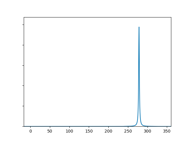
Admittedly, it isn’t the most exciting spectrum, with a single peak around 280 cm-1. Let’s make some adjustments: we’ll add a touch more Gaussian broadening, zoom in on the peak by limiting the axis range, add axis labels and write to a file.
galore test/CaF2/ir_lda_700.txt -g 1.2 -l  --spikes \
  --plot ir_lda_700_better.png \
  --xmin 200 --xmax 350 --units cm-1 --ylabel Intensity
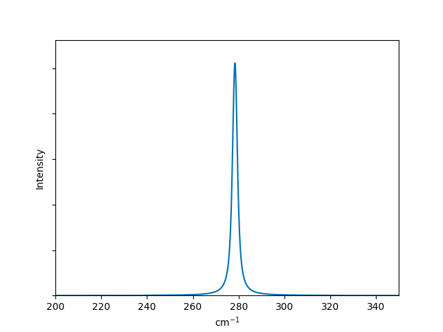
Now the plot is more publication-ready! If you would like to use
another plotting program, the broadened data can be output to a CSV
file by simply replacing --plot with --csv:
galore test/CaF2/ir_lda_700.txt -g 1.2 -l -k --csv --xmin 200 --xmax 350
(Here we have also replaced --spikes with its short form -k.)
This will write a csv file to the standard output as no filename was
given. We can also write space-separated text data, so for example
galore test/CaF2/ir_lda_700.txt -g 1.2 -l -k --txt ir_CaF2_broadened.txt
generates a file with two columns (i.e. energy and broadened intensity).
Simulated Raman
Broadening a simulated Raman spectrum is very similar to broadening a simulated IR spectrum. Galore recognises the output format of the vasp_raman.py code, which automates the process of following vibrational modes and calculating the polarisability change on each displacement. The output file has a simple format and Galore recognises them by inspecting the header. Sample data is included (computed with LDA using VASP with a 500 eV cutoff) as test/CaF2/raman_lda_500.dat. We generate a plot in the same way as before:
galore test/CaF2/raman_lda_500.dat -g -l -k --plot --units cm-1 --ylabel Intensity --style Solarized_Light2
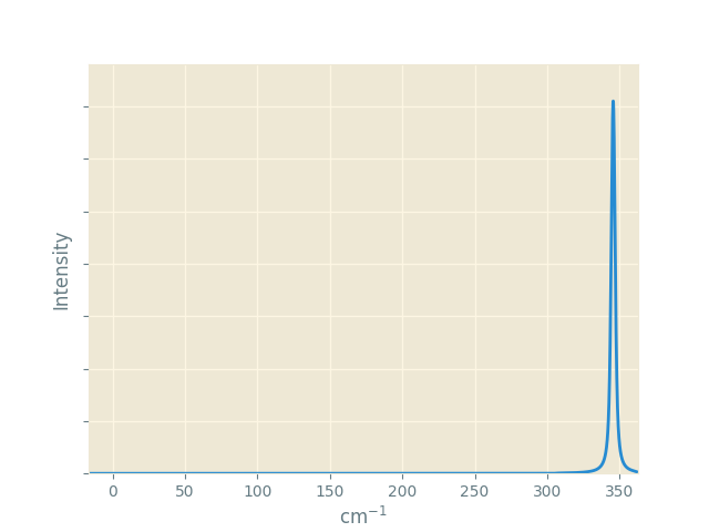
This time we set an alternative appearance style with --style Solarized_Light2.
Galore uses Matplotlib styles, and you can use inbuilt styles or create custom stylesheets.
The dark_background style may be useful for slide presentations.
Note that for the same material we are seeing a single peak again, but
at a different frequency to the IR plot. This is not a shift; the peak
at 280 cm-1 is still present but has zero activity, while the
peak calculated at 345 cm-1 has zero IR activity.
Simulated Photoelectron Spectroscopy
Photoelectron measurements allow valence band states to be probed fairly directly; energy is absorbed by an incident photon as it ejects an electron from the sample, and the shift in energy is measured relative to a monochromatic photon source. Ultraviolet photoelectron spectroscopy (UPS), x-ray photoelectron spectroscopy (XPS) and Hard x-ray photoelectron spectroscopy (HAXPES) are fundamentally similar techniques, differing in the energy range of the incident photons.
These binding energies may be compared with the full density of states (DOS) computed with ab initio methods. However, the intensity of interaction will vary depending on the character of the energy states and the energy of the radiation source. The relevant interaction parameter (“photoionization cross-section”) has been calculated systematically over the periodic table and relevant energy values; Galore includes some such data from Yeh and Lindau (1985).
In ab initio codes it is often possible to assign states to particular orbital characters; often this is limited to s-p-d-f (i.e. the second quantum number) but in principle an all-electron code can also assign the first quantum number. Directional character is also sometimes assigned, usually relative to Cartesian axes. These various schemes are used to construct a “projected density of states” (PDOS).
The construction of a PDOS in ab initio calculations is slightly arbitrary and lies beyond the scope of Galore. However, when the orbital assignment has been made the DOS elements can be weighted to simulate the photoionization spectrum.
We begin by plotting a PDOS from sample data in test/MgO. This was computed using VASP with standard pseudopotentials and the revTPSS exchange-correlation functional.
galore test/MgO/MgO_Mg_dos.dat test/MgO/MgO_O_dos.dat \
  --plot --pdos -g 0.5 -l 0.2 --ylabel DOS --units eV
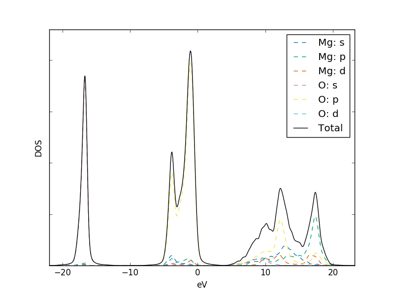
Note that the --pdos flag is required to enable the reading of
orbital-projected input files. The element identity is read from
these filenames, and is expected between two underscore
characters. The orbital names are determined from the column headers
in this file.
It is possible to use spin-polarised data by using a header form such
as ‘s(up)’ and ‘s(down)’ for spin-polarised s-orbitals, in which case
the contributions of the spin channels will be summed together.
Let’s turn this into a useful XPS plot. The flag --weightings can
be used to pass a data file with cross-section data; for some cases
data is build into Galore. Here we will use the data for Al k-α
radiation which is denoted alka is built into Galore. We also flip
the x-axis with --flipx to match the usual presentation of XPS
data as positive ionisation or binding energies rather than the
negative energy of the stable electron states. Finally the
data is written to a CSV file with the --csv option.
galore test/MgO/MgO_Mg_dos.dat test/MgO/MgO_O_dos.dat \
  --plot mgo_xps.png --pdos -g 0.2 -l 0.2 --weighting alka \
  --units ev --xmin -1 --xmax 8 --ylabel Intensity \
  --csv mgo_xps.csv --flipx
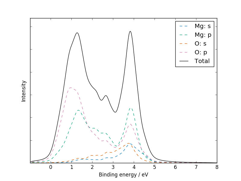
Plotting the CSV file with a standard plotting package should give a similar result to the figure above; if not, please report this as a bug!
Compare with literature: tin dioxide
Sample VASP output data is included for rutile tin dioxide. This was computed with the PBE0 functional, using a 4x4x5 k-point mesh and 700 eV basis-set cutoff. The structure was optimised to reduce forces to below 1E-3 eV Å-1 using 0.05 eV of Gaussian broadening and the DOS was computed on an automatic tetrahedron mesh with Blöchl corrections. Instead of the separate .dat files used above, we will take advantage of Galore’s ability to read a compressed vasprun.xml file directly. This requires the Pymatgen library to be installed:
pip3 install --user pymatgen
If the GPAW Python library is available, it is also possible to import this data from .gpw output files.
XPS
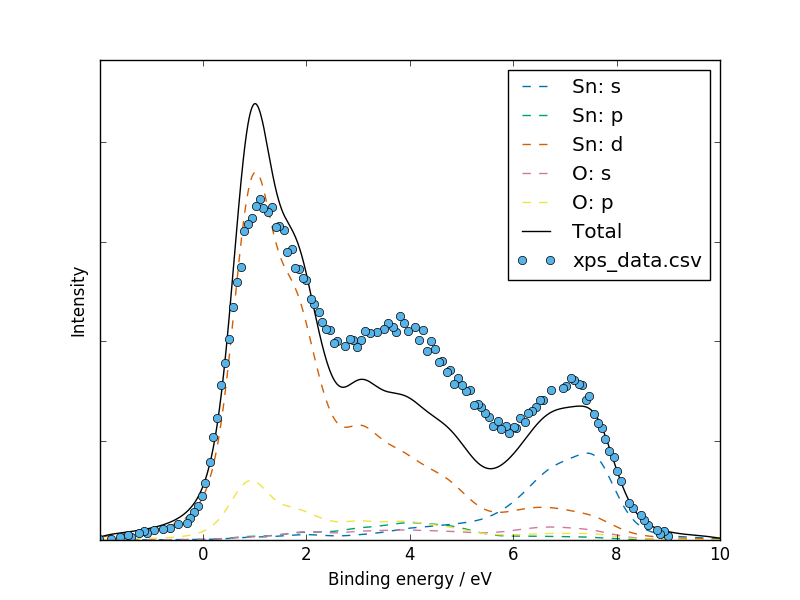
We have digitised the experimental data plotted in Fig.3 of Farahani et al. (2014) in order to aid a direct comparison:
galore test/SnO2/vasprun.xml.gz --plot -g 0.5 -l 0.4 \
  --pdos --w alka --flipx --xmin -2 --xmax 10 \
  --overlay test/SnO2/xps_data.csv  --overlay_offset -4 \
  --overlay_scale 5 --units ev --ylabel Intensity
(Note that here the shorter alias -w is used for the XPS
weighting.) The general character and peak positions match well, but
the relative peak intensities could be closer; the first peak is very
strong even with cross-section weightings applied. We can see that the
dip in between the second an third main peak corresponds to a crossing
point between the contributions of the Sn-s and Sn-d orbitals.
A slightly more generous assignment of ‘p’ vs ‘d’ character by the orbital projection scheme would have made for a better fit! The published results seem to fit better despite using similar calculation parameters; we can’t see if the orbital breakdown is indeed the determining factor.
UPS
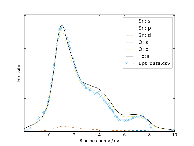
Experimental UPS data was digitized from Fig. 1 of Themlin et al. (1990). A satisfactory fit is obtained for the three main peaks, but the “bump” below zero suggests the presence of some phenomenon in the bandgap which was not captured by the ab initio calculation:
galore test/SnO2/vasprun.xml.gz --plot -g 0.5 -l 0.9 \
  --pdos --w he2 --flipx --xmin -2 --xmax 10 \
  --overlay test/SnO2/ups_data.csv --overlay_offset 0.44 \
  --units ev --ylabel Intensity --overlay_style x
The authors noted this in their own comparison to a DOS from tight-binding calculations:
The location of the VBM in out UPS data was complicated by the presence of a slowly varying photoelectron signal, resulting from a surface-state band.
HAXPES
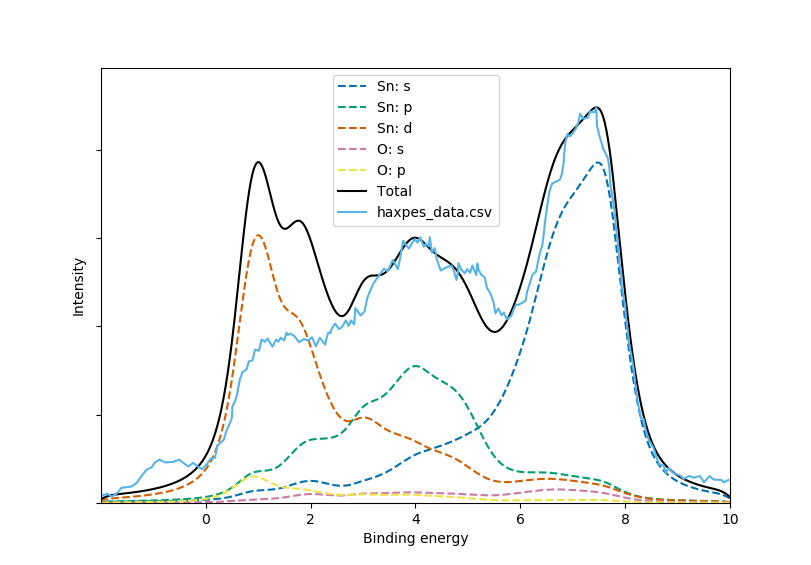
A HAXPES spectrum was obtained by digitizing Fig. 1 of Nagata et
al. (2011). These experiments
were performed with 5.95 keV x-rays; we set --w 5.95 to estimate
corresponding cross-sections by fitting to
Scofield (1973):
galore test/SnO2/vasprun.xml.gz --plot -g 0.3 -l 0.5 --pdos \
  --w 5.95 --flipx --xmin -2 --xmax 10 \
  --overlay test/SnO2/haxpes_data.csv --overlay_offset -3.7 \
  --ylabel Intensity --overlay_style -
We see that the weighting goes some way to rebalancing the peak intensities but once again the Sn-d states are over-represented. Surface states above the valence band are seen in the experimental data.
Python API
The Python API allows custom plots to be produced by generating data sets Galore’s core functions and passing Matplotlib axes to the plotting functions. A few examples are provided below. It is not especially difficult to access the lines plotted to an axis and manipulate their appearance, rescale them etc.
Overlaying different amounts of broadening
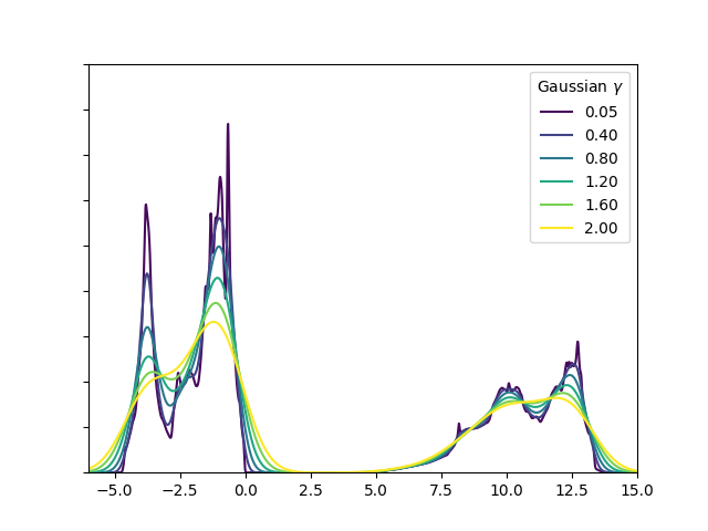
1 2 3 4 5 6 7 8 9 10 11 12 13 14 15 16 17 18 19 20 21 22 23 24 25 26 27 28 29 30 31 32 33 34 | #! /usr/bin/env python3
import numpy as np
import matplotlib.pyplot as plt
from matplotlib.cm import viridis as cmap
import galore
import galore.plot
vasprun = 'test/MgO/vasprun.xml.gz'
xmin, xmax = (-6, 15)
fig = plt.figure()
ax = fig.add_subplot(1, 1, 1)
widths = np.arange(0, 2.01, 0.4)
widths[0] = 0.05 # Use a finite width in smallest case
for g in widths:
x_values, broadened_data = galore.process_1d_data(input=vasprun,
gaussian=g,
xmin=xmin, xmax=xmax)
broadened_data /= g # Scale values by broadening width to conserve area
galore.plot.plot_tdos(x_values, broadened_data, ax=ax)
line = ax.lines[-1]
line.set_label("{0:2.2f}".format(g))
line.set_color(cmap(g / max(widths)))
ax.set_ylim(0, 1800)
legend = ax.legend(loc='best')
legend.set_title('Gaussian $\gamma$')
plt.show()
|
Plotting different amounts of broadening on tiles
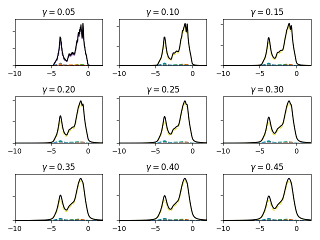
1 2 3 4 5 6 7 8 9 10 11 12 13 14 15 16 17 18 19 20 21 22 23 | #! /usr/bin/env python3
import numpy as np
import matplotlib.pyplot as plt
plt.style.use("seaborn-colorblind")
import galore
import galore.plot
vasprun = './test/MgO/vasprun.xml.gz'
xmin, xmax = (-10, 2)
fig = plt.figure()
for i, l in enumerate(np.arange(0.05, 0.50, 0.05)):
ax = fig.add_subplot(3, 3, i + 1)
ax.set_title("$\gamma = {0:4.2f}$".format(l))
plotting_data = galore.process_pdos(input=[vasprun], lorentzian=l,
xmin=xmin, xmax=xmax)
galore.plot.plot_pdos(plotting_data, ax=ax)
ax.legend().set_visible(False)
fig.tight_layout()
plt.show()
|
Comparing different photoemission weightings
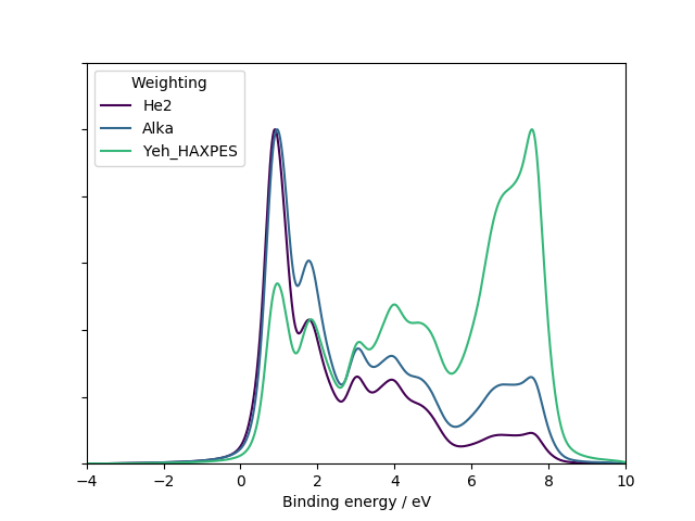
1 2 3 4 5 6 7 8 9 10 11 12 13 14 15 16 17 18 19 20 21 22 23 24 25 26 27 28 29 30 31 32 33 34 35 36 | #! /usr/bin/env python3
import numpy as np
import matplotlib.pyplot as plt
from matplotlib.cm import viridis as cmap
import galore
import galore.plot
vasprun = 'test/SnO2/vasprun.xml.gz'
xmin, xmax = (-10, 4)
fig = plt.figure()
ax = fig.add_subplot(1, 1, 1)
weightings = ('He2', 'Alka', 'Yeh_HAXPES')
for i, weighting in enumerate(weightings):
plotting_data = galore.process_pdos(input=[vasprun],
gaussian=0.3, lorentzian=0.2,
xmin=xmin, xmax=xmax,
weighting=weighting)
galore.plot.plot_pdos(plotting_data, ax=ax, show_orbitals=False,
units='eV', xmin=-xmin, xmax=-xmax,
flipx=True)
line = ax.lines[-1]
line.set_label(weighting)
line.set_color(cmap(i / len(weightings)))
ymax = max(line.get_ydata())
line.set_data(line.get_xdata(), line.get_ydata() / ymax)
ax.set_ylim((0, 1.2))
legend = ax.legend(loc='best')
legend.set_title('Weighting')
plt.show()
|